It’s 02:17, your phone buzzes. pg_stat_statements says query f8472a91 has a mean runtime of 6.2 seconds over the last hour. The raw text is a six-table join with a couple of sub-selects. You copy it, paste it into a psql session, slap EXPLAIN (ANALYZE, BUFFERS) on front, and get a tight index scan that finishes in 80 ms. The plan in production looked nothing like this. Between the page-out of the original data, the buffer cache being warm now, and stats changing on the fly, you’re chasing a ghost. I walk through exactly this scenario in a companion video — the gap between “this query is slow” and “here is why” can swallow half your night.
📖 Read the full guide: auto_explain: Turning “My query is slow” from a guessing game into a captured cr
▶ Watch the video walkthrough: auto_explain: Catching Slow Plans in the Act
https://www.youtube.com/watch?v=hfO4kuhu32k
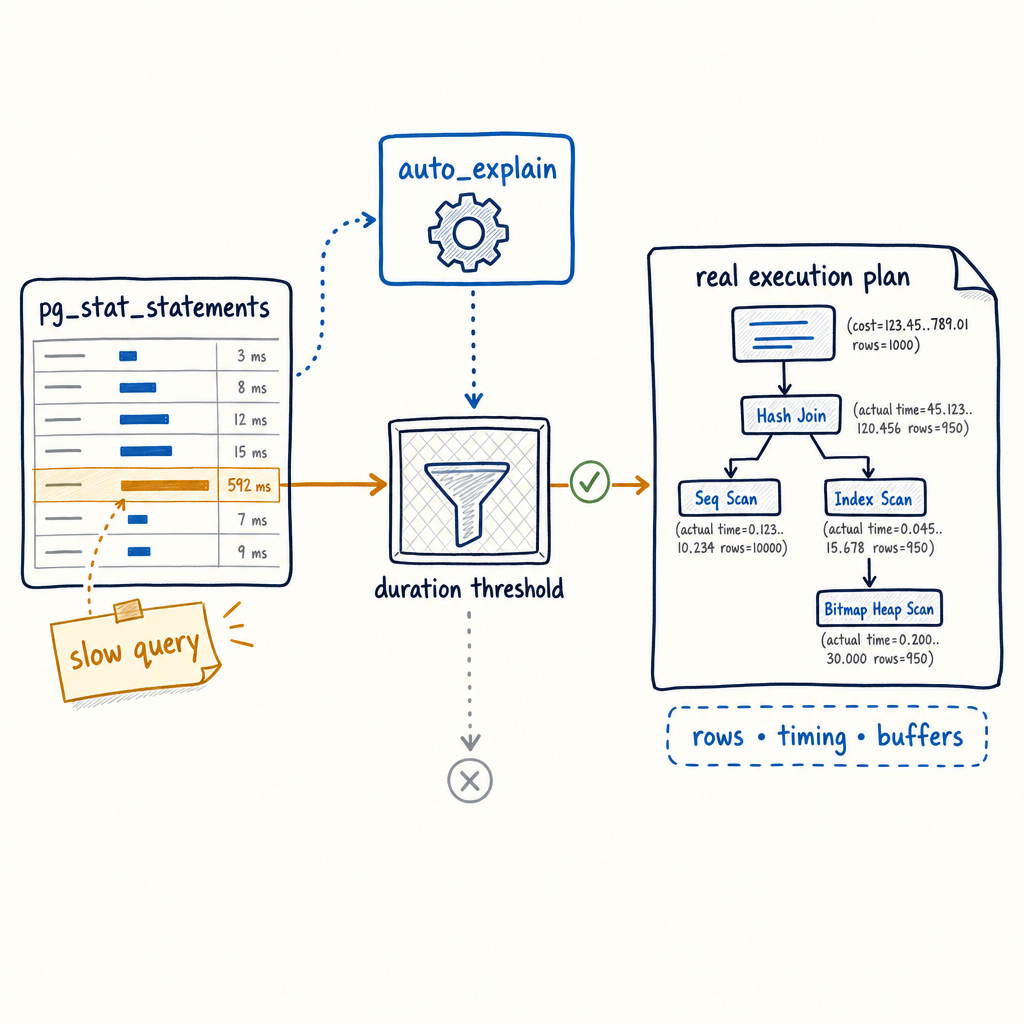
auto_explain closes that gap. It hooks into the executor and writes the real execution plan — with actual row counts, per-node timing, and buffer usage — straight to the PostgreSQL log the moment a query exceeds your chosen duration threshold. No manual reproduction, no stale snapshot, no speculation.
What auto_explain does (and doesn’t) do
auto_explain is a contrib module that sits inside the executor. Every time a statement finishes, Postgres checks the elapsed wall-clock time. If that time crossed auto_explain.log_min_duration, the module logs the plan. With auto_explain.log_analyze = on, it logs the actual execution statistics — the very same output you’d get from EXPLAIN (ANALYZE, BUFFERS, TIMING). This includes true row counts, per-node timing, and buffer hit/miss counts for shared, local, and temp buffers. The output lands in the server log, timestamped and attached to the session that ran the query. You get the plan as it happened, not as you hoped it would.
It doesn’t replace pg_stat_statements. That extension still gives you normalized query fingerprints, aggregate call counts, and total time. But pg_stat_statements cannot show you how a specific execution traversed its relations or where the estimation went wrong. auto_explain fills that hole.
Installing and enabling it
Because auto_explain is a shared library, it must be loaded at server start — a simple pg_reload_conf() won’t cut it. You need a full restart.
Add auto_explain to shared_preload_libraries. If you’re already using pg_stat_statements, the line in postgresql.conf looks like:
shared_preload_libraries = 'pg_stat_statements, auto_explain'
Or use ALTER SYSTEM:
ALTER SYSTEM SET shared_preload_libraries = 'pg_stat_statements, auto_explain';
Then restart the server:
pg_ctl restart -D /path/to/data
After the restart, verify:
SHOW shared_preload_libraries;
SELECT * FROM pg_available_extensions WHERE name = 'auto_explain';
You’ll see auto_explain in the list. The module is present but not yet active — you still need to set its configuration parameters.
The core knobs, one by one
All configuration lives under the auto_explain. namespace. Here are the parameters with their defaults and my recommended starting point for a busy production system:
| Parameter | Default | Recommended | What it does |
|---|---|---|---|
auto_explain.log_min_duration |
-1 (off) |
2000 (2 sec) |
Log plans for queries that run longer than this many milliseconds. Set to 0 to log everything (dangerous). |
auto_explain.log_analyze |
off |
on |
Include actual row counts, per-node timing, and buffers. Without this you only get the estimated plan, which is rarely what you need at 2am. |
auto_explain.log_buffers |
off |
on |
Add buffer usage counts (shared hit/read/dirtied, local, temp). Essential for spotting cache-churn queries. |
auto_explain.log_timing |
on |
on |
Include per-node startup and total time. Keep it on unless you profile sub-millisecond queries at high frequency. |
auto_explain.log_verbose |
off |
off |
Adds output columns and schema-qualified names. Turn on only when you need the extra detail (it bloats the log). |
auto_explain.log_triggers |
off |
off |
Include trigger execution statistics. Enable if you’re troubleshooting trigger-heavy workloads, otherwise off. |
auto_explain.log_nested_statements |
off |
on (if you have functions) |
Log plans for statements executed inside functions and procedures. Without this, the expensive query inside a PL/pgSQL loop stays invisible. |
auto_explain.log_format |
text |
text |
Output format: text, json, xml, yaml. Stick with text unless you’re piping logs to a tool that parses structured formats. |
auto_explain.sample_rate |
1.0 |
0.1 |
Fraction of qualifying queries to log. At 0.1, only 10% of slow queries are recorded — enough to catch pattern repeats while keeping overhead negligible. |
Here’s a copy-paste block for postgresql.conf (after the restart already loaded the library):
auto_explain.log_min_duration = 2000
auto_explain.log_analyze = on
auto_explain.log_buffers = on
auto_explain.log_timing = on
auto_explain.log_triggers = off
auto_explain.log_verbose = off
auto_explain.log_nested_statements = on
auto_explain.log_format = text
auto_explain.sample_rate = 0.1
Apply with SELECT pg_reload_conf(); — no restart needed because the library is already loaded; the rest are standard SIGHUP-able GUCs. Keep in mind that while the extension itself demands a full restart, every auto_explain.* parameter can be changed and applied with a simple configuration reload.
Reading real output: a misestimate caught in the act
Let’s look at an actual log entry that got me out of bed one night. The query was a simple select over orders joined with order_lines, filtered on a status column and a date range. pg_stat_statements told me this thing had a mean time of 8500 ms. When I ran it manually, it used a nice index scan and returned in 62 ms. Here’s what auto_explain wrote to the log during the slow execution (I’ve truncated the plan for space):
2025-04-07 02:23:11 UTC [16384]: [2-1] user=app,db=orders_db LOG:  duration: 8472.341 ms  plan:
	Query Text: SELECT o.order_id, o.customer_id, sum(l.quantity * l.unit_price)
	FROM orders o JOIN order_lines l ON o.order_id = l.order_id
	WHERE o.status = 'pending' AND o.order_date >= now() - interval '30 days'
	GROUP BY o.order_id, o.customer_id;
	Aggregate  (cost=54293.12..54318.12 rows=1000 width=24) (actual time=8472.321..8472.331 rows=3842 loops=1)
	  ->  Nested Loop  (cost=1.29..54243.08 rows=10000 width=16) (actual time=0.445..8467.112 rows=847293 loops=1)
	        ->  Seq Scan on orders o  (cost=0.00..2215.08 rows=50 width=8) (actual time=0.030..42.581 rows=847293 loops=1)
	              Filter: ((status = 'pending') AND (order_date >= (now() - '30 days'::interval)))
	              Rows Removed by Filter: 15623
	        ->  Index Scan using order_lines_pkey on order_lines l  (cost=1.29..1.38 rows=200 width=20) (actual time=0.008..0.009 rows=1 loops=847293)
	              Index Cond: (order_id = o.order_id)
	Planning Time: 1.203 ms
	Execution Time: 8472.431 ms
The planner estimated 50 rows from orders after the filter. The executor got 847,293. That drove a nested loop instead of the hash join we’d expect, and it ran for 8.4 seconds. You don’t need to squint: the row estimate is off by a factor of 16,945. The Seq Scan was the wrong choice.
What do you do next?
- Check statistics freshness.
ANALYZE orders;might bring the histogram up to date if thependingstatus exploded recently. - Increase the statistics target for the filtered columns.
ALTER TABLE orders ALTER COLUMN status SET STATISTICS 1000;gives the planner more sample resolution. - If status and order_date are correlated (e.g., recent orders are more likely pending), the planner’s independence assumption bites you. Create extended statistics:
CREATE STATISTICS orders_status_date (dependencies) ON status, order_date FROM orders;
ANALYZE orders;
- If the predicate remains selective most of the time, a partial index can give the planner a cheap access path:
CREATE INDEX CONCURRENTLY orders_pending_recent_idx ON orders (order_date)
WHERE status = 'pending';
The log excerpt gave you exact numbers to quantify the damage and pick a fix. Without it, you’d be guessing.
Overhead: why log_analyze isn’t free and how sample_rate fixes it
When auto_explain.log_analyze = on, Postgres enables instrumentation for every node in the plan tree of every query that could potentially exceed the threshold. It’s not just a switch flipped retroactively. The executor has to insert timing calls (gettimeofday() or equivalent) at each node start and end, count rows, and track buffer pin/unpin stats. On a tight OLTP workload running thousands of queries per second, this constant timing overhead can add 2–5% CPU load, sometimes more if the plan has many nodes. That’s why blindly turning on full analysis for every query is reckless.
sample_rate decouples the overhead from the visibility. Set sample_rate = 0.1 and you only instrument 10% of queries that cross log_min_duration. Because the slow queries are the ones you care about, a 10% sample will catch the repeating bad plans quickly — if a query blips once, it might escape, but if it hammers the database for an hour, you’ll get dozens of samples. Meanwhile, the 90% of fast queries never invoke the extra instrumentation on slow-path code, keeping the steady-state overhead near zero.
Start with sample_rate = 0.1 and log_min_duration = 2000ms. For high-QPS systems, think in terms of captures per minute: with 10,000 queries per second, 2% of them might exceed 2 seconds (200 slow queries/sec). A 0.1 sample rate gives 20 logged plans per second, which is plenty. If you’re on a smaller instance doing 200 queries per second, you might raise sample_rate to 1.0 because you’ll see one slow query every few seconds anyway. Adjust down only if the log volume becomes noisy.
Where the logs go and how to actually use them
The plans land in the main PostgreSQL log stream. If you use the standard logging collector (logging_collector = on), they’ll appear under log_directory, typically pg_log inside the data directory. Check with:
SHOW log_directory;
SHOW log_filename;
To extract them, grep for plan: and look for preceding duration: lines to find the long runners:
grep -B1 "plan:" postgresql-2025-04-07.csv | grep "duration: [89][0-9]\{3,\}"
That finds plans with durations 8000 ms or more. You can pipe the output to a dedicated slow‑plan log file for periodic review, or attach -A 50 to grab the full multi‑line plan block behind each match:
grep -B1 "plan:" postgresql-*.csv | grep "duration: [89][0-9]\{3,\}" \
  | cut -d' ' -f-2 > slow_plans_this_week.txt
Automate this with a cron job, and you’ll have a running list of the worst plans delivered to your inbox every morning.
Why auto_explain belongs in every production cluster
After the first time auto_explain hands you the exact row miscount that turned a 60‑ms look‑up into a 9‑second table scan, you’ll wonder why you ever ran a database without it. The library adds negligible overhead when you keep sample_rate conservative, and the data it captures—true execution plans with true row counts—transforms the 2‑AM firefight from wild speculation into a structured, evidence‑based fix. Combine it with pg_stat_statements for the aggregate view and you have a complete diagnostics stack. Set the knobs once, document the log location for your on‑call team, and sleep better knowing that the next time a query goes sideways, the real plan will already be waiting in the logs.